Tutorial Archives - 1stVision Inc. - Machine Vision Articles

June 1, 2026June 2, 2026

HDR in machine vision – solving bright and dark imaging challenges

High dynamic range (HDR) isn’t new. It’s frequently mentioned. And offered on-camera, or via software or FPGA. Is it just a marketing term, or a real benefit? If your application’s scenes contain both bright and dark regions, HDR can absolutely deliver benefits.

Consider the three images shown below:

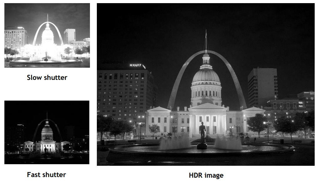
Neither the “slow shutter” image nor the “fast shutter” image is optimal. The former is over-saturated – one can’t even find the many windows in the central building. The fast shutter image is of course too dark, essentially losing the arch and the flagpole. While this scene is more from the realm of “photography” than “machine vision”, the concepts are the same.

Clearly the best image is the HDR image – the lighter areas are revealed in nuanced detail, but so too the unlit trees and gray windows are clear in their own degrees of black and gray, and everything in between. How is this achieved?

What is HDR?

Let’s unpack the acronym, starting with DR for dynamic range. DR is the ratio between the largest and smallest measurable values, for the quantity being measured. For machine vision, it’s light intensity that’s being quantified.

Generally speaking, a larger dynamic range is preferrable to a small one, as the nuanced differences of a relatively larger dynamic range may be required for effective image processing. Take edge-detection, a common machine vision requirement for many applications. The edge may only become apparent, under given lighting conditions and resolution, when the saturation of pixels in a given region are consistently lower to one side and consistently higher to the other side of the “emergent” edge. With sufficient dynamic range, calculated confidence grows, while poor dynamic range may fail to reveal an edge at all.

Ways to create a composite HDR image

One way to create an HDR image is with two exposures and an algorithm for creating the composite. The shorter exposure captures the more brightly lit or highly reflective surfaces, while the remaining regions remain unsaturated or only slightly registering. A longer exposure oversaturates the lighter targets, but reveal nuanced variation in the previously unrevealed details.

In fact one does the longer exposure first, such that the darker portions of the scene produce a variance of non-zero values – i.e. a dynamic range across the darker regions.

Then for the shorter exposure, use the brightest non-saturated pixels from the first exposure as a reference to generate small non-zero values as a control on the short exposure, creating a calculated point of overlap. That way many pixels that were oversaturated on the long exposure are only slightly to moderated saturated on the short-exposure, for a nuanced spread of values across the corresponding pixels.

The blending algorithm compares the two images, pixel for pixel, with the overlap point as a reference. Saturated pixels in the first image are replaced with the corresponding non-saturated pixel values from the second image.

While the two-exposure approach described above is easy to understand, there’s clearly a time-cost in taking two successive exposures, reading them both out to the PC host, and doing the image processing. For certain applications, that may be acceptable. For others, especially with motion involved, or desired high cycle counts, one might hope for a faster approach.

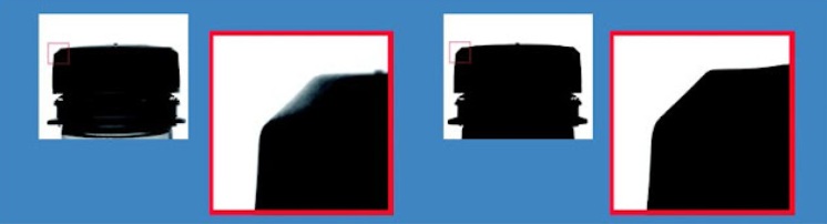
Another way: multi-slope pixel generation on CMOS sensors

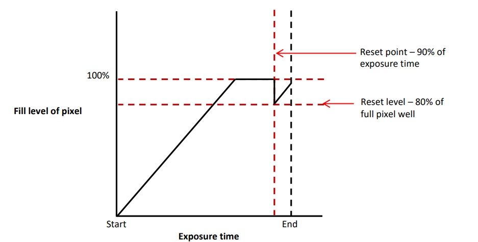
The rise of CMOS sensors and their transistor-based pixel architecture enables on-sensor functionality that convenient supports the generation of HDR images. This may be achieved by resetting pixels approaching saturation, prior to end of exposure, so those pixels have an opportunity to be filled from a range of values instead of maxing out had the reset not occurred.

Consider the follow two diagrams, and the supporting discussion below:

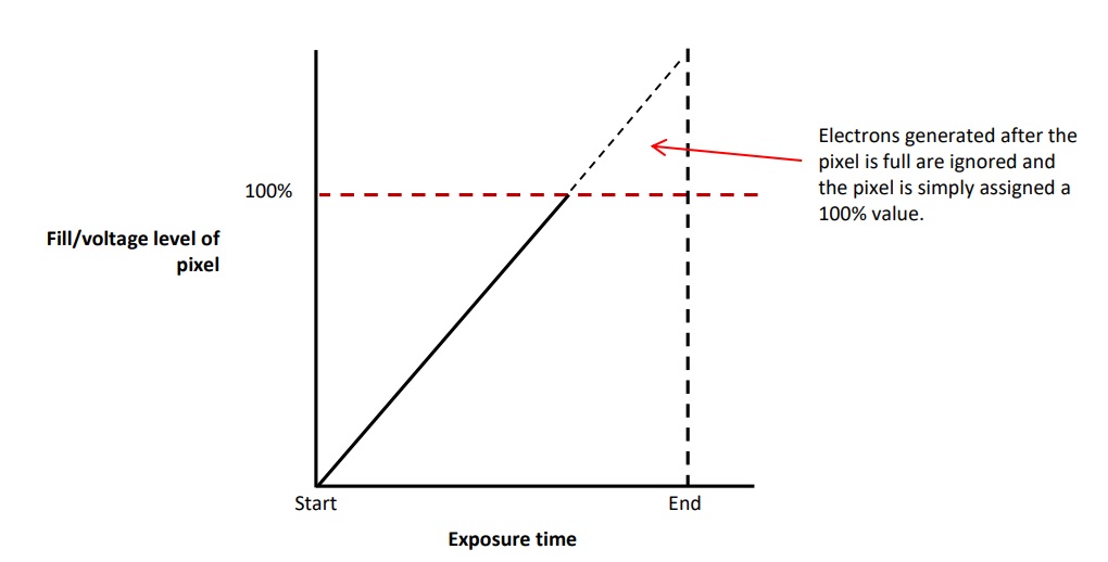
If many pixels fill before the end of the exposure, a lot of the image may be oversaturated, even though the darker regions need a longer exposure to become meaningfully non-zero. Courtesy JAI.

But thanks to CMOS transistors at each pixel position, the sensor can be programmed to monitor saturation values, and to reset pixels approaching saturation to “partial fill” levels that allow additional fill for the remainder of the exposure.

It gets even better

Above was “intro level” HDR, concepts and techniques that provide the foundation. Meanwhile innovators keep taking it to the next level.

For example, Sony now offers Quad HDR on their IMX900 sensor, available in the IDS uEye low-cost cameras. Getting the dark sections sufficiently saturated while not oversaturating the brighter regions is really evident with Quad HDR below.

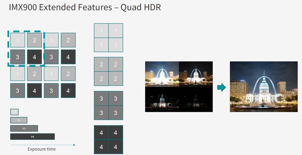
Quad HDR generates a balanced image – Courtesy IDS

In the video below, you may jump to position 1 minute 42 seconds for more on Quad HDR:

Even more on HDR:

If you’d like to read a more in-depth treatment on HDR, including more example images, supporting arithmetic and graphical rational, download our whitepaper on High Dynamic Range Imaging.

Or perhaps you have an application with known nuanced dark regions as well as variation in the saturated areas, for which HDR may add value. Should you do it on-camera/sensor? In an FPGA/frame-grabber? On the PC host? Use lighting techniques to avoid needing HDR altogether? There are a number of different ways to achieve optimal image outcomes, but HDR is certainly a valuable technique for some applications.

Call us at 978-474-0044, and let us guide you to a best-fit solution.

1st Vision’s sales engineers have over 100 years of combined experience to assist in your camera and components selection. With a large portfolio of cameras, lenses, cables, NIC cards and industrial computers, we can provide a full vision solution!

About you: We want to hear from you! We’ve built our brand on our know-how and like to educate the marketplace on imaging technology topics… What would you like to hear about?… Drop a line to info@1stvision.com with what topics you’d like to know more about.

#HDR

#Highdynamicrange

June 4, 2025June 4, 2025

Collimated lighting important with telecentric lens

LTCLHP Collimated Light – Courtesy Opto Engineering

Machine vision practitioners, regardless of application or lens type, know that contrast is essential. Without sharp definition, features cannot be detected effectively.

When using a telecentric lens for precision optical 2-D measurements, ideally one should also use collimated lighting. Per the old adage about a chain being only as good as its weakest link, why invest in great lensing and then cut corners on lighting?

WITH collimated light expect high edge definition:

The cost of the light typically pays for itself relative to quality outcomes. Below see red-framed enlargements of the same region of a part being imaged by the same telecentric lens.

The left-hand image was taken with a conventional backlight – note how the light wraps around the edge, creating “confusion” and imprecision due to refracted light coming from all angles.

The right-hand image was obtained with a collimated backlight – with excellent edge definition.

Conventional backlight (left) vs. collimated backlight (right) – Courtesy Opto Engineering.

It all comes down to resolution

While telecentric imaging is a high-performance subset of the larger machine vision field in general, the same principles of resolution apply. It takes several pixels to confidently resolve any given feature – such as an edge – so any “gray areas” induced by lower quality lighting or optics would drag down system performance. See our blog and knowledge-base coverage of resolution for more details.

Collimated lighting in more detail

Above we see the results of using “diffuse” vs. “collimated” light sources, which are compelling. But what is a collimated light and how does it work so effectively?

UNLIKE a diffuse backlight, whose rays emanate towards the object at angles ranging from 0 to almost 180°, a collimated backlight sends rays with only very small deviations from perfectly parallel. Since parallel rays are also all that the telecentric lens receives and transmits on to the camera sensor, stray rays are mitigated and essentially eliminated.

The result is a high-contrast image which is easier to process with high-reliability. Furthermore, shutter speeds are typically faster, achieving necessary saturation more quickly, thereby shortening cycle times and increasing overall throughput.

Many lights to choose from:

The video below shows a range of light types and models, including clearly labeled direct, diffuse, and collimated lights.

Several light types – including clearly labeled collimated lights

[Optional] Telecentric concepts overview

Below please compare the diagrams that show how light rays travel from the target position on the left, through the respective lenses, and on to the sensor position on the far right.

A telecentric lens is designed to insure that the chief rays remain parallel to the optical axis. The key benefit is that (when properly focused and aligned) the system is invariant to the distance of the object from the lens. This effectively ignores light rays coming from other angles of incidence, and thereby supports precise optical measurement systems – a branch of metrology.

If you’d like to go deeper on telecentrics, see the following two resources:

Telecentric concepts presented as a short blog.

Alternatively as a more comprehensive Powerpoint from our KnowledgeBase.

Video: Selecting a telecentric lens:

Call us at 978-474-0044 to tell us more about your application – and how we can guide you through telecentric lensing and lighting options.

February 23, 2025February 24, 2025

How to calculate line rate on a line scan camera based on conveyor speed

Unless one calculates and sets the line rate correctly, there’s a risk of blur and sub-optimal performance. And/or purchasing a line scan camera that’s not up to the task; or that’s overkill and costs you more than would have been needed.

Line Scan concept – Courtesy Teledyne DALSA

Optional line scan review or introduction

Skip to the next section if you know line scan concepts already. Otherwise…

Perhaps you know about area scan imaging, where a 2D image is generated with a global shutter, exposing all pixels on a 2D sensor concurrently. And you’d like to understand line scan imaging by way of comparing it to area scan. See our blog What is the difference between an Area Scan and a Line Scan Camera?

30 minute informative overview of Line Scan imaging – Courtesy Teledyne DALSA

Maybe you prefer seeing a specific high-end product overview and application suggestions, such as the Teledyne DALSA 16k TDI line scan camera with 1MHz line rate. Or a view to tens of different line scan models, varying not only by manufacturer, but by sensor size and resolution, interface, and whether monochrome or color.

Either you recall how to determine resolution requirements in terms of pixel size relative to defect size, or you’ve chased the link in this sentence for a tutorial. So we’ll keep this blog as simple as possible, dealing with line rate calculation only.

Line scan cameras – Courtesy Teledyne DALSA

Calculate the line rate

Getting the line rate right is the application of the Goldilocks principle to line scanning.

Line rate too slow…	Line rate too fast…
Blurred image if due to too long exposure, and/or missed segments due to skipped “slices”	Oversampling can create confusion by identifying the same feature as two distinct features

Why we need to get the line rate rate right

A rotary encoder is typically used to synchronize the motion of the conveyor or web with the line scan camera (and lighting if pulsed). Naturally the system cannot be operated faster than the maximum line speed, but it may sometimes operator more slowly. This may happen during ramp up or slow down phases – when one may still need to obtain imaging – or by operator choice to conserve energy or avoid stressing mechanical systems.

Naming the variables … with example values

Resolution A = object space correlation to sensor; FOV / pixel array; e.g. if 550mm FOV and 2k sensor = 550/2000 = 0.275 pixels per mm

Transport speed T = mm per sec; e.g. 4k / 1mm yields rate of motion

Sampling frequency F = T / A; for example values above F = 4000 / 0.275 = 14545.4545 = 14.5kHz; spelled out: Frequency = Transport_speed / Pixel_spatial_resolution (what 1 pixel equals in target space)

For the example figures used above, a line scan camera with 2k resolution and a line scan frequency of about 14.5 kHz will be sufficient.

Download spreadsheet with labeled fields and examples:

Just click here, or on the image below, to download the spreadsheet calculator. It includes clearly labeled fields, and examples, as the companion piece for this blog:

Not included here… but happy to show you how

We’ve kept this blog intentionally lean, to avoid information overload. Additional values may also be calculated, of course, such as:

Data rate in MB / sec: Useful to confirm camera interface can sustain the data rate

Frame time: The amount of time to process each scanned image. Important to be sure the PC and image processing software are up to the task – based on empirical experience or by conferring with software provider.

January 20, 2025January 22, 2025

Explained: Trifecta of lens f-stop, wavelength and Airy disc

In this blog we tackle a set of issues well-known to experts. It’s complex enough to be non-obvious, but easy enough to understand through this short tutorial. And better to learn via a no-cost article rather than through trial and error.

Alternative to reading on, let us help you get the optics right for your application. Or read on and then let us help you anyway. Helping machine vision customers choose optimal components is what we do. We’ve staked our reputation on it.

Click here for help from 1stVision

Aperture size and F-stop

Most understand that the F-stop on a lens specifies the size of the aperture. Follow that last link to reveal the arithmetic calculations, if you like, but the key thing to keep in mind at the practical level is that F-stop values are inversely correlated with the size of the aperture. So a large F-number like f/8 indicates a narrow aperture, while a small F-number like f/1.4 corresponds to a large aperture. Some lens designs span a wider range of F-numbers than others, but the inverse correlation always applied.

Iris controls the aperture – Courtesy Edmund Optics

Maximizing contrast might seem to suggest a large aperture

For machine vision it’s always important to maximize contrast. The target object can only be discerned when it is sufficiently contrasted against the background or other objects. Effective lighting and lensing is crucial, in addition to a camera sensor that’s up to the task.

“Maximizing light” (without over-saturating) is often a challenge, unless one adds artificial light. That would tend to suggest using a large aperture to let more light pass while still keeping exposure time short enough to “freeze” motion or maximize frames per second.

So for the moment, let’s hold that thought that a large aperture sounds promising. Spoiler alert: we’ll soften our position on this point in light of forthcoming points.

Depth of Field – DoF

While a large aperture seems attractive so far, one argument against that is depth of field (DoF). In particular, the narrowest effective aperture maximizes depth of field, while the largest aperture minimizes DoF.

Correlation of aperture size and depth of field – Courtesy Edmund Optics

Depending on the lens design, the difference in DoF between largest vs. smallest aperture may vary from as little as a few millimeters to as great as many centimeters. Your applications knowledge will inform you how much wiggle room you’ve got on DoF.

So what’s the sweet spot for aperture?

Barring further arguments to the contrary, the largest aperture that still provides sufficient depth of field is a good rule of thumb.

Where do diffraction limits and the Airy disc come into it?

Optics is a branch of physics. And just like absolute zero in the realm of temperature, Boyle’s law with respect to gases, etc., there are certain constraints and limits that apply to optics.

Whenever light passes through an aperture, diffraction occurs – the bending of waves around the edge of the aperture. The pattern from a ray of light that falls upon the sensor takes the form of a bright circular area surrounded by a series of weakening concentric rings. This is called the Airy disk. Without going into the math, the Airy disk is the smallest point to which a beam of light can be focused.

And while stopping down the aperture increases the DoF, our stated goal, it has the negative impact of increasing diffraction.

Correlation of aperture to diffraction pattern – Courtesy Edmund Optics

Diffraction limits

As focused patterns, containing details in your application that you want to discern, near each other, they start to overlap. This creates interference, which in turn reduces contrast.

Every lens, no matter how well it is designed and manufactured, has a diffraction limit, the maximum resolving power of the lens – expressed in line pairs per millimeter. There is no point generating an Airy disk pattern from adjacent real-world features that are larger than the sensor’s pixels, or the all-important contrast needed will not be achieved.

And wavelength’s a factor too?

Indeed wavelength is also a contributor to contrast and the Airy disc. As beings who see, we tend to default to thinking of light as white light or daylight, which is a composite segment of the spectrum, from indigo, blue, green, yellow, orange, and red. That’s from about 380 nm to 780 nm. Below 380 nm we find ultraviolet light (UV) in the next segment of the spectrum. Above 780 nm the next segment is infrared (IR).

Monochrome light better than white light

An additional topic relative to the Airy disc is that monochrome light is better than white light. When light passes through a lens, it refracts (bends) differently in correlation with the wavelength. This is referred to as chromatic aberration.

Transverse and longitudinal chromatic aberration – Courtesy Edmund Optics

If a given point on your imaged object reflect or emits light in two more more of the wavelengths, the focal point of one might land in a different sensor pixel than the other, creating blur and confusion on how to resolve the point.

An easy way to completely overcome chromatic aberration is to use a single monochromatic wavelength! If your target object reflects or emits a given wavelength, to which your sensor is responsive, the lens will refract the light from a given point very precisely, with no wavelength-induced shifts.

Need help to get all parts optimized? Speak with a sales engineer. Click here to request a callback.

Or call us at 978-474-0044

The moral of the story

The takeaway point is that the trifecta of aperture (F-stop) and wavelength each have a bearing on the Airy disc, and that one wants to choose and configure the optics and lighting to optimize the Airy disc. This leads to effective applications performance – a must have. But it can also lead to cost-savings, as lower cost lenses, lighting, and sensors, optimally configured, may perform better than higher cost components chosen without sufficient understanding of these principles.